

Enterprise AI infrastructure has shifted from optimizing training models to serving them, and that changes the economics. Training is a capital project with an endpoint. Inference is a production workload that runs as long as the service is live, with output measured in tokens. This is the tokenomics problem now facing AI operators: once the GPUs are racked and the power budget is set, the business depends on how many tokens the hardware produces.
In long, multi-turn workloads, the same context is repeatedly passed through the model as conversations grow. The GPU already paid to process those tokens once, but when the KV cache is evicted, the system has to prefill that context again. That makes the enemy recompute. At any scale, that is not a rounding error. It is expense handed back as power, GPU time, queue growth, or additional hardware.
The reflexive fix is to buy more of the most expensive resources in the rack: more GPUs, more DRAM. But recompute has already produced something reusable. The KV cache is just data; it can be stored and retrieved cheaply, trading a small reload cost for the expensive prefill computation it avoids. The question then is not whether to keep the cache, but where to keep it, and that is as much a cost question as a performance one. VRAM is the fastest tier and the scarcest; once it saturates, the inference server starts evicting caches. DRAM buys headroom at a steep and rapidly rising price. Flash is where the math can change: slower than DRAM, certainly, but far less expensive per terabyte, with enough capacity to hold the context the faster tiers are forced to discard, which is the difference between reprocessing the whole conversation and simply reading it back.
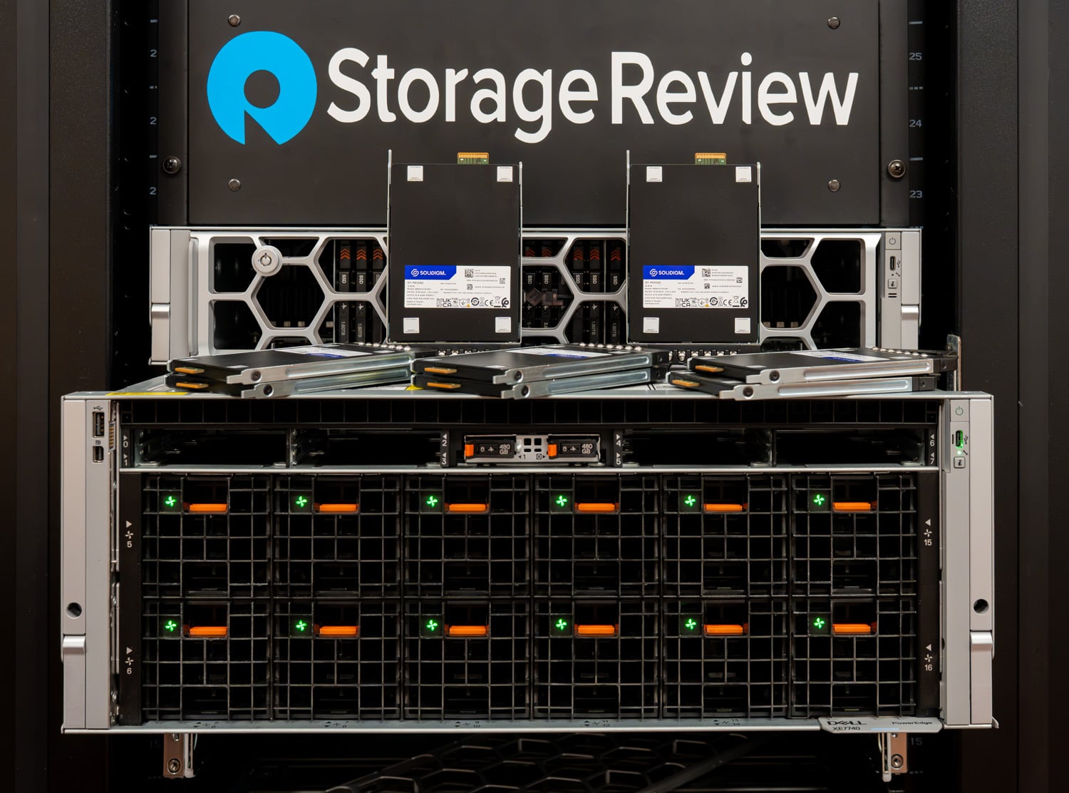
To measure the impact, we built a multi-turn agentic test workload on a Dell PowerEdge XE7740 and held the model, GPUs, and serving stack constant. The number that matters for anyone sizing a system is what happens after the memory tiers fill. Past that point, flash sustained roughly 30,000 total tokens per second, compared with DRAM’s 17,000, holding 94% of its own peak while the DRAM tier fell to 42%. Both offload tiers beat the VRAM-only baseline by a wide margin at peak (2.9X on DRAM and 2.2X on flash), but the peak is precisely where the DRAM tier is about to run out. The most expensive memory buys the peak; flash holds it as the context keeps growing.
Before getting into the results, it is worth being precise about what the KV cache is, why it fills up, and why inference performance starts to collapse when the system has nowhere cheaper to keep it.
Key Takeaways
- Flash sustains what DRAM cannot: All three configurations perform identically until memory pressure forces eviction. VRAM saturates first, and the 512GB DRAM tier fills roughly 45 minutes into the run and begins evicting. Past that point flash sustains about 30,000 total tokens per second against DRAM’s 17,000, holding 94% of its own peak while DRAM fell to 42%.
- Offload recovers throughput lost to recompute: At peak, KV cache offload raised total serving throughput up to 2.9X over the VRAM-only baseline on the DRAM tier and 2.2X on flash. The gain comes from skipping re-prefill, since context the GPU already computed is read back from the offload tier rather than rebuilt.
- Returning users feel the difference most: Worst-case first-token latency on a resumed session was 13.9 seconds on the VRAM-only baseline against 3.2 seconds on flash. Offload is what keeps that tail inside a bound an interactive user will sit through.
- Agentic traffic makes eviction expensive: A week of instrumented Claude Code traffic was 98.16% cache reads, with just 0.02% genuinely cold input.
- KV offload is a write-heavy workload that demands high-endurance drives: Every token the model produces writes a KV entry, and TTL churn keeps rewriting the tier around the clock. At our sustained write rate, the mirrored RAID10 array we tested works out to roughly 3.2 drive writes per day per drive, dropping to about 1.6 DWPD striped as RAID0, bracketing the D7-PS1030’s 3 DWPD rating. Endurance, not capacity or speed, is the defining constraint of the flash tier, and because the cache is disposable, working a write-focused drive this hard is an acceptable trade.
How Inference Works
Large language models are autoregressive: each output token is conditioned on every token that came before it. The attention mechanism implements that conditioning by computing (for each token in the sequence) a query (Q) vector that is matched against the key (K) and value (V) vectors of every prior token. The attention output is a weighted combination of the values, with the weights coming from the Q-K dot products.
When a request arrives, the prompt cannot be answered until the K and V tensors exist for every token in it. That first step is prefill: the engine runs the prompt through the model in a single parallel pass and writes the resulting K and V tensors to memory. Prefill is thus compute-bound, and its latency scales with prompt length.
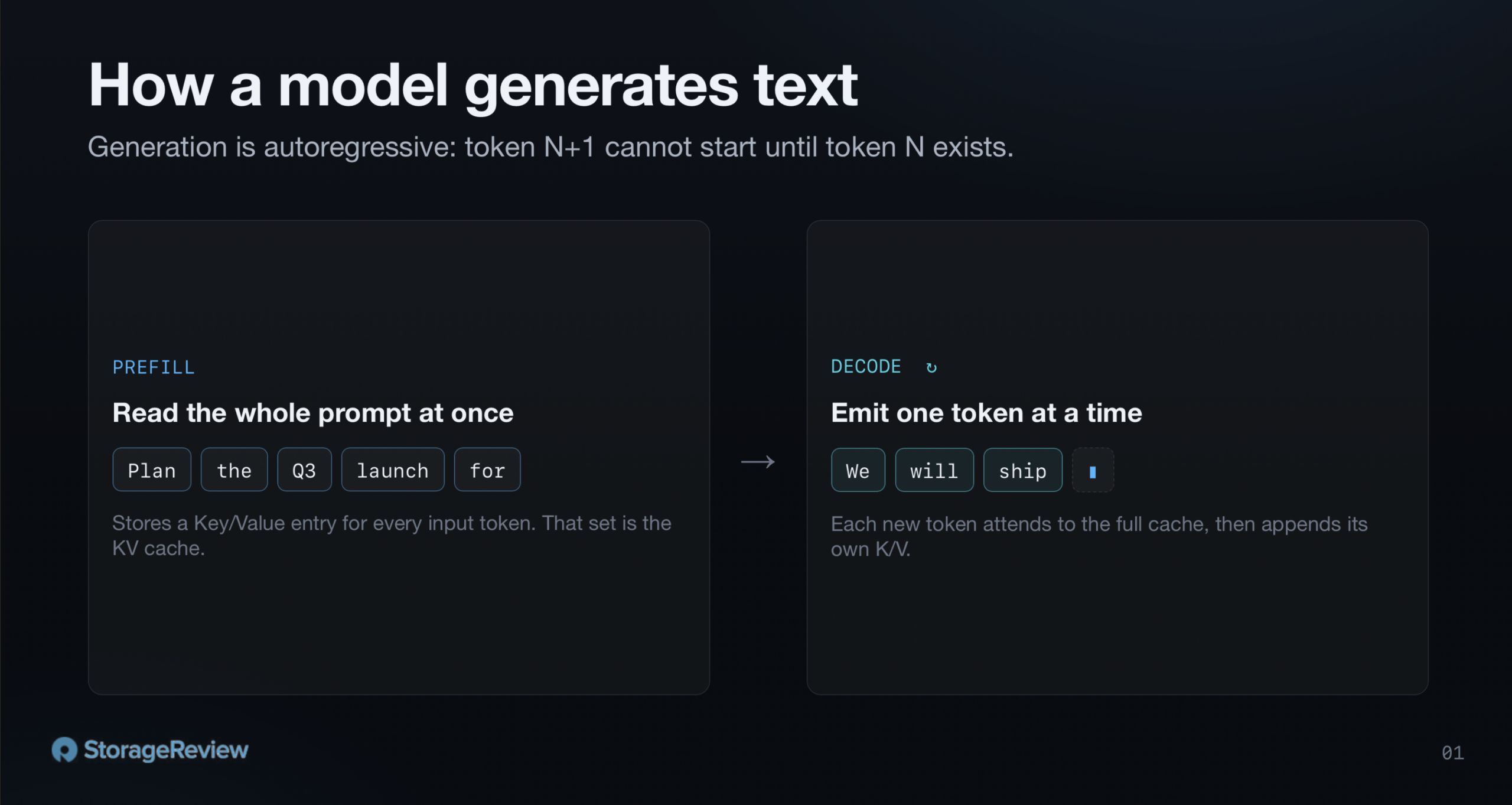
Once prefill finishes, the engine emits the response one token at a time. Each new token reads back the K and V of every prior token, computes its attention output, and writes its own K and V into memory for the next step. That second phase is decode. It is sequential and memory-bandwidth-bound because generating each token requires loading the cached K and V tensors for all prior tokens from memory and computing attention over them before writing the new token’s K and V tensors for future steps.
The K and V tensors from both phases are the KV cache. Without them, generating the n+1th token would recompute the keys and values for all n prior tokens at every step, which is quadratic in compute complexity. With the cache in place, each new token computes only its own K and V and reads the rest from memory, so the per-token cost stays linear.
What Agentic Traffic Looks Like
People often describe inference as memory-bandwidth-bound because decode dominates the user-visible portion of a response. The actual balance between the two phases is workload-dependent. A short prompt requesting a long essay is decode-heavy; a long agentic prompt requesting a small JSON edit is prefill-heavy. Which side dominates determines what gets stressed when the cache is mismanaged.
The shape of the recompute problem follows from that balance, and “agentic” covers a wide range of usage patterns. Agentic coding is one of the most popular of those patterns right now, and on the OpenRouter leaderboards, it accounts for a significant portion of tokens used. To quantify a representative case, we instrumented Claude Code with OpenTelemetry (OTEL) logging and exported a week’s worth of traces to Grafana. The breakdown of that token traffic by type is shown below. Note: This Claude Code usage is on the Claude Opus 4.8 model with 1M context length, working on multiple coding projects at once.
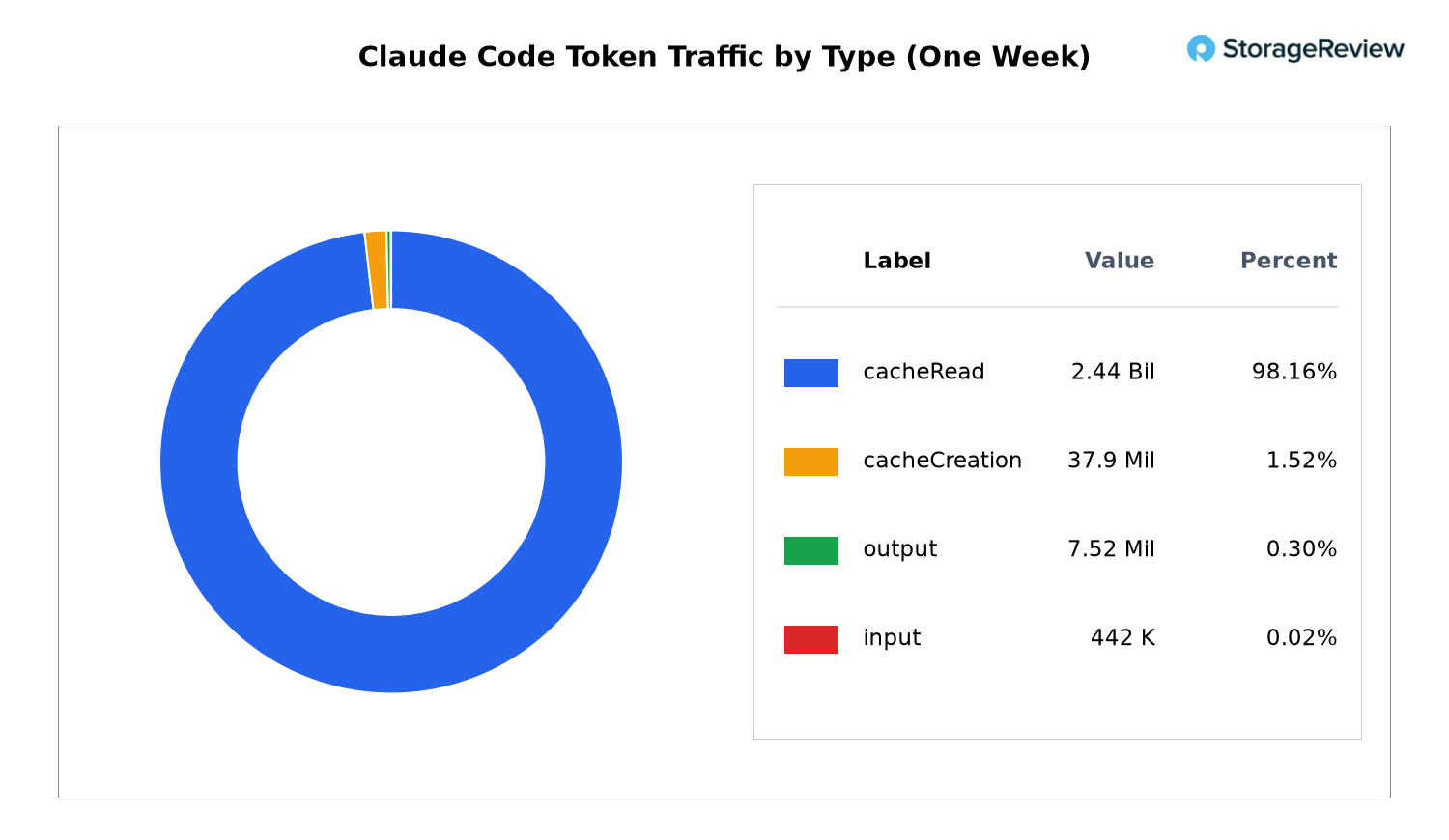
Cache reads accounted for 98.16% of all token traffic. Cache creation (a previously seen prefix being re-prefilled because its entry had expired) was 1.52%. Output tokens were 0.30%. Genuinely cold input tokens were 0.02%.
In a workload where 98% of traffic is cache reads, eviction without offload means re-prefilling the bulk of the work the system was about to do. The bottleneck shifts from decode bandwidth, which is the phase typically optimized, to prefill compute, which the GPU already performed in earlier turns. In fact, it is quite common to see disaggregated serving architectures running more prefill workers than decode workers at scale for the same reason: prefill is the gating phase.
The 98% figure is one user’s traffic mix. A short-turn chat workload would show more cold traffic. A retrieval-augmented system that re-injects different documents per turn would too. The general shape holds wherever conversations are long, prefixes are stable, and users keep returning to the same context.
Where the Cache Lives, and What Happens When It Fills
Where does this cache actually live, and what happens when it runs out of room? After the model weights load, any remaining VRAM becomes KV cache space, partitioned into fixed-size blocks, and at startup the engine tells you how many tokens it can hold. That pool is the only place the cache can live in a standard setup without KV Offloading.
GPU servers are expensive, and tokens are the product, so the goal is to keep them fed around the clock. That means keeping the GPU loaded with a small queue of requests waiting to be processed so compute doesn’t sit idle, while balancing the queue to keep response latency within the service-level-objective (SLO). Not every request will consume its full context window, so many completed KVs stay cached in VRAM on their own. But under sustained load, that cache fills up, and once it does, older entries get evicted to make room.

In an ideal world, you would one-shot every answer and be done with it. But models are not that good yet, so we run agentic loops, turning back and forth with a user or between agents. When the next turn arrives, if its KV is not yet cached, the engine reprocesses the entire conversation so far, plus the new tokens. Every prior turn’s context is run through the model again, and the computation the GPU already did on those tokens is paid for a second, third, and subsequent times for every subsequent turn. This part of the exercise is pure waste.
What KV Cache Offload Changes
Instead of evicting the moment VRAM fills, offload progressively spills caches down a hierarchy: VRAM to system memory to SSD. The hot working set stays in VRAM; entries that no longer fit are pushed to system memory, and if system memory fills up, they are pushed again to the SSD or a networked storage tier. Real eviction becomes rare, driven by a user-set time-to-live (TTL) rather than by memory pressure.
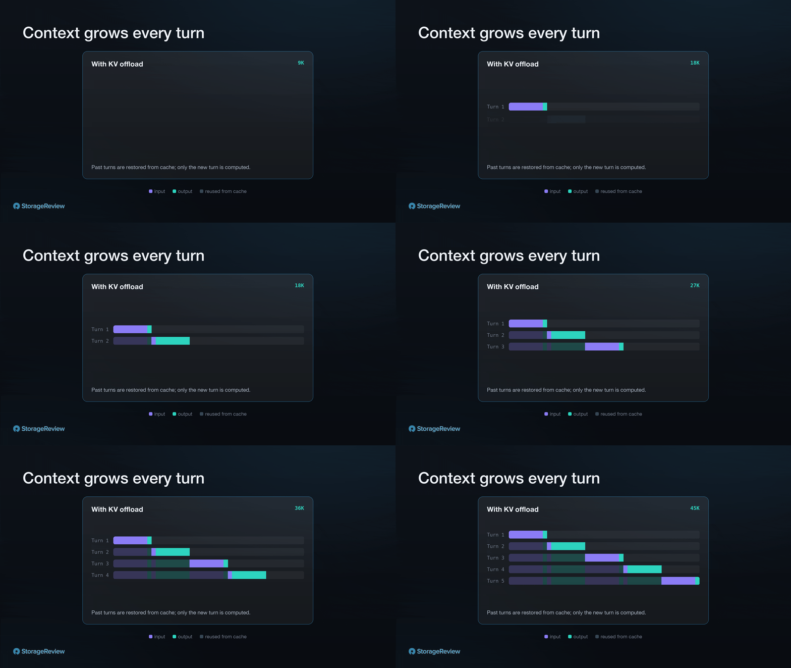
When that next turn lands, instead of recomputing tens of thousands of tokens of context, we pull the KV back from RAM or flash storage instead. Reloading from system memory incurs a small latency penalty but is far cheaper and faster than redoing the prefill. Reloading from NVMe is a bit slower than a DRAM fetch, but still much faster than the recompute it replaces. Storage capacity is relatively inexpensive; GPU compute is not, so trading a little reload latency at the start of a turn to skip a multi-second recompute is net positive.
How We Tested
We put this to the test in our lab. The system configuration was as follows:
- Server: Dell PowerEdge XE7740
- GPUs: 4x NVIDIA RTX PRO 6000 Blackwell Server Edition (96GB)
- System memory: 1TB DDR5 (16 x 64GB 5200MT/s DDR5)
- Storage: 8x Solidigm PS1030 12.8TB E3.S Drives (RAID10)
- Serving stack: vLLM 0.22.0 with LMCache 0.5.0
- Model: MiniMax-M2.7
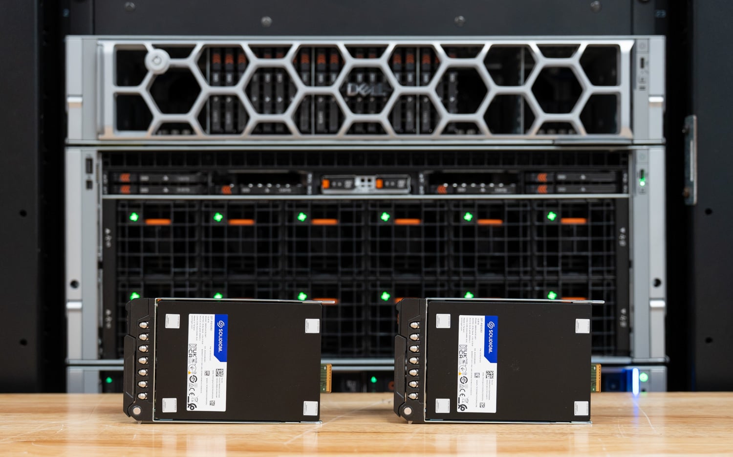
The test platform is a perfect fit for this workload. Dell’s PowerEdge XE7740 is purpose-built for enterprise AI inference, a PCIe Gen5 chassis that supports up to 8 double-wide GPUs. The four-GPU configuration we ran is one of the most popular configurations sold. It provides enough accelerator capacity for a broad range of inference deployments while leaving room in the same box to scale to eight as demand grows. Each NVIDIA RTX PRO 6000 Blackwell Server Edition contributes 96GB of GDDR7 memory, so four cards stand up a substantial pool of VRAM before any cache has to leave the GPU. Underneath, the offload tier rides on eight 12.8TB Solidigm D7-PS1030 drives in RAID10, Gen5 high-endurance flash suited to the sustained writes a KV cache tier generates. And finally, the model choice, MiniMax-M2.7 was, at the time of testing, one of the top open coding models that fit within our four-GPU configuration.
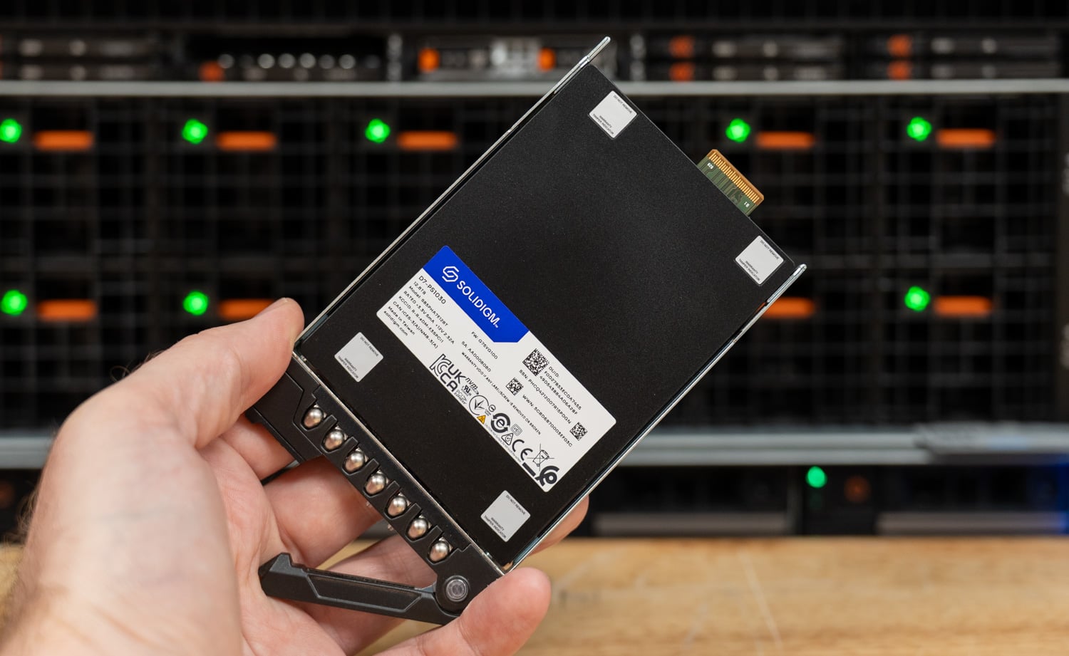
We tested three configurations:
- A VRAM baseline, stock vLLM with no offload, where whatever fits in VRAM is cached, and everything else evicts.
- LMCache offloading to system memory, with 512GB allocated for offload.
- LMCache offloading to flash, with the local RAID10 NVMe array as the offload tier, fronted by a 64GB RAM staging buffer.
We modeled the workload on real agentic coding traffic rather than a fixed synthetic prefix sweep. That traffic is prefill-heavy and decode-light, with extensive prefix reuse. Sessions arrive as a Poisson process at a rate of λ = 2.5 sessions per minute. Each session runs over multiple turns. On each turn, the model takes in a short append, usually a tool or command result of 250 to 600 tokens, and occasionally a 1,500 to 3,500-token file read. It replies with a short response, usually 40 to 200 tokens of tool calls or brief reasoning, and occasionally a 400 to 900-token code block. Turn lengths are jittered by ±100 tokens. Sessions grow monotonically toward a 64k-token context ceiling, which puts them in the deep-context regime, where the working set outgrows VRAM. The same seeded load drives all three tiers, each with a 3-minute cache warm-up.
Quick note on the memory config: the XE7740 as shipped came loaded with 2TB of DDR5, a top-spec build meant to cover a range of projects, and priced before the 2026 memory run-up made that much DRAM a very different line item. The original configuration was over-spec’d relative to what an organization would order today with four GPUs, so to make it more realistic, we removed 1TB of memory, leaving one DIMM per channel to preserve maximum memory throughput.
One methodology note on the flash tier: the runs used LMCache’s local disk backend with its required 64GB RAM staging buffer in front of the array. The KV footprint retained on flash grew well beyond the host’s total DRAM over the course of the run, so the sustained results reflect drive service rather than host memory.
Performance
Throughput under Load
Total serving throughput over the run, as the KV working set grows past what each tier can hold:
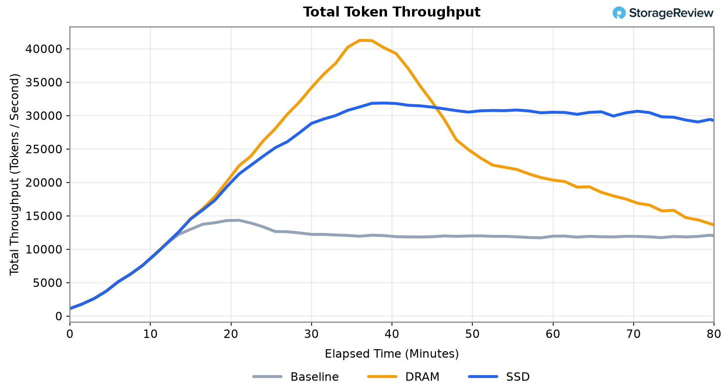
Every tier ramps up together for the first 10 minutes while the caches are still filling, with basically no difference in performance. Then, as the memory tiers fill up, they separate. The VRAM-only baseline stalls first: once VRAM saturates, it plateaus around 12,000 total tokens per second. Each new session evicts an older one, and the displaced cache must be rebuilt from scratch when that session returns, so more of every second goes to re-prefill, and less to decode.
The DRAM and SSD tiers keep climbing well past that plateau because, until their caches fill, they serve nearly every prefix from memory or disk rather than recomputing it. The time the baseline burns on re-prefill goes into generating new tokens instead.
At peak, offload delivered up to 2.9X the baseline’s total serving throughput on the DRAM tier (+188%) and 2.2X on the flash tier (+122%). Before the working set outgrows VRAM, all three configurations land within a percent of each other. Nothing evicts, so there is nothing for offload to recover. The benefit appears only when memory pressure forces eviction, and it grows with the degree to which the server is pushed.
The case for a larger tier shows up once DRAM fills. At this load, the 512 GB RAM cache saturates roughly 45 minutes into the run, and from there it has to start evicting. Returning prefixes miss and get re-prefilled, the exact recompute the cache was meant to avoid. The SSD tier, with terabytes of headroom, never hits that wall. Past the crossover, flash sustains about 30,000 total tokens per second, compared to DRAM’s roughly 17,000, a 75% throughput advantage for SSD once RAM runs out. Put another way, after saturating, the DRAM tier delivered just 42% of its peak throughput, while the SSD tier delivered 94% of its own. This is the capacity ladder the whole exercise turns on: VRAM runs out first, the 512 GB DRAM tier runs out later, and a storage tier measured in terabytes rather than gigabytes effectively never runs out, so it keeps serving context long after the faster tiers have had to start throwing it away.
One caveat on reading that total-throughput number: the tens of thousands of tokens per second it reports are not the rate at which the GPUs compute tokens; in large part they are the offload tier’s serving rate. Total throughput counts every input prefill token plus every output decode token each request carries. But with the cache in place, a hit loads the prefix’s KV back from DRAM or flash instead of re-prefilling it on the GPU.
Restricting the count to output tokens, the part of the throughput a user actually waits on, gives a cleaner picture:
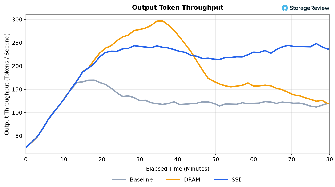
On output tokens, the three tiers again track together while the caches are filling, then split at the crossover. The DRAM tier peaks near 300 tokens per second, a 75% increase over the baseline, and slides back as it starts to evict; flash holds near 250 through the rest of the run, a 46% increase over the baseline. The RAM and SSD lines stay within roughly 10% of each other until DRAM saturates; after that, the gap widens.
First-Token Latency: What the User Waits On
Throughput measures aggregate token production. Time-to-first-token measures what an individual user sees: the wait from hitting send to the first token coming back. We plot it over the run, at the median, as the working set grows and each tier fills.
While the caches hold, all three tiers return a first token in about half a second. Then they diverge, in the same order their throughput did. The baseline breaks first: it climbs past 10 seconds early in the run, while the DRAM tier stays under 1-second TTFT for much longer, until its 512 GB fills around the 45-minute mark. Then its latency cliffs as it begins evicting and recomputing. The SSD tier degrades the most gently and holds the lowest tail of the three across the back half of the run.
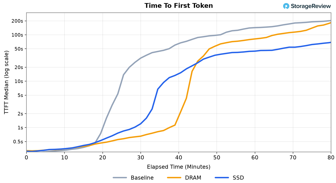
That flip is the tiering argument in miniature. DRAM is the latency winner while the working set fits in that tier; flash is the latency winner once it does not, because it still holds context the DRAM tier has begun throwing away.
The Returning-User Problem
The latency numbers above cover turns within a continuous session. The returning-user case is different: a session pauses mid-conversation, sits idle for about fifteen minutes, then picks up where it left off. We modeled it with a cohort that went dormant after roughly 20 turns and was revived 15 minutes later, long enough for a busy server to cycle other traffic through its caches in the meantime. Eleven such revivals landed inside each tier’s measurement window, and because the workload is seeded identically across tiers, the same eleven sessions revived in every run, giving a like-for-like comparison of the resume turn. The chart below plots each tier’s median first-token time on a normal turn against the resume turn, with the whisker marking the worst resume in the sample.
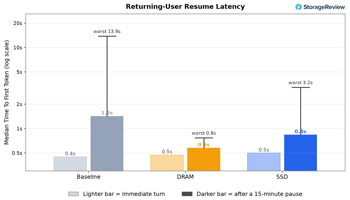
At the median, the numbers only confirm what the mechanics predict, and the tiers land in the expected order. DRAM leads: a dormant session resumes in 0.6 seconds, barely above the 0.5 seconds a normal turn takes. SSD is second at 0.8 seconds; we know an NVMe fetch is slower than a DRAM fetch, and that’s part of what peeks through here. The VRAM-only baseline is slowest at 1.4 seconds; with nothing to offload to, the idle session’s prefix was evicted from GPU memory for live traffic, and the first turn back has to recompute it. At best, the whole spread is only about a second.
The best case is not the one where the choice is made. The worst of the eleven revivals in each tier is: 0.8 seconds on DRAM, 3.2 seconds on SSD, and 13.9 seconds on the baseline. Whether a fourteen-second wait for a first token is tolerable or a hard SLO violation depends on the service, but for anything interactive it is the latter, and only the offload tiers keep that tail inside a bound a user will sit through. It also widens in context, since recompute cost scales with how much history the returning user has built up: at the deeper contexts of the throughput test, the baseline tail runs well past 14 seconds, while DRAM and SSD still incur only a bounded reload.
Choosing and Sizing the KV Cache
Both offload tiers beat the VRAM-only baseline by a wide margin, and they land close to each other on the way there. The gap is small because the throughput win is just VRAM being freed, and the same amount gets freed whether the evicted cache lands in DRAM or on SSD. Throughput does not care which tier the cache came back from. Latency does, since a DRAM fetch is faster than an NVMe fetch, but both are cheap next to recomputing the same KV from scratch.
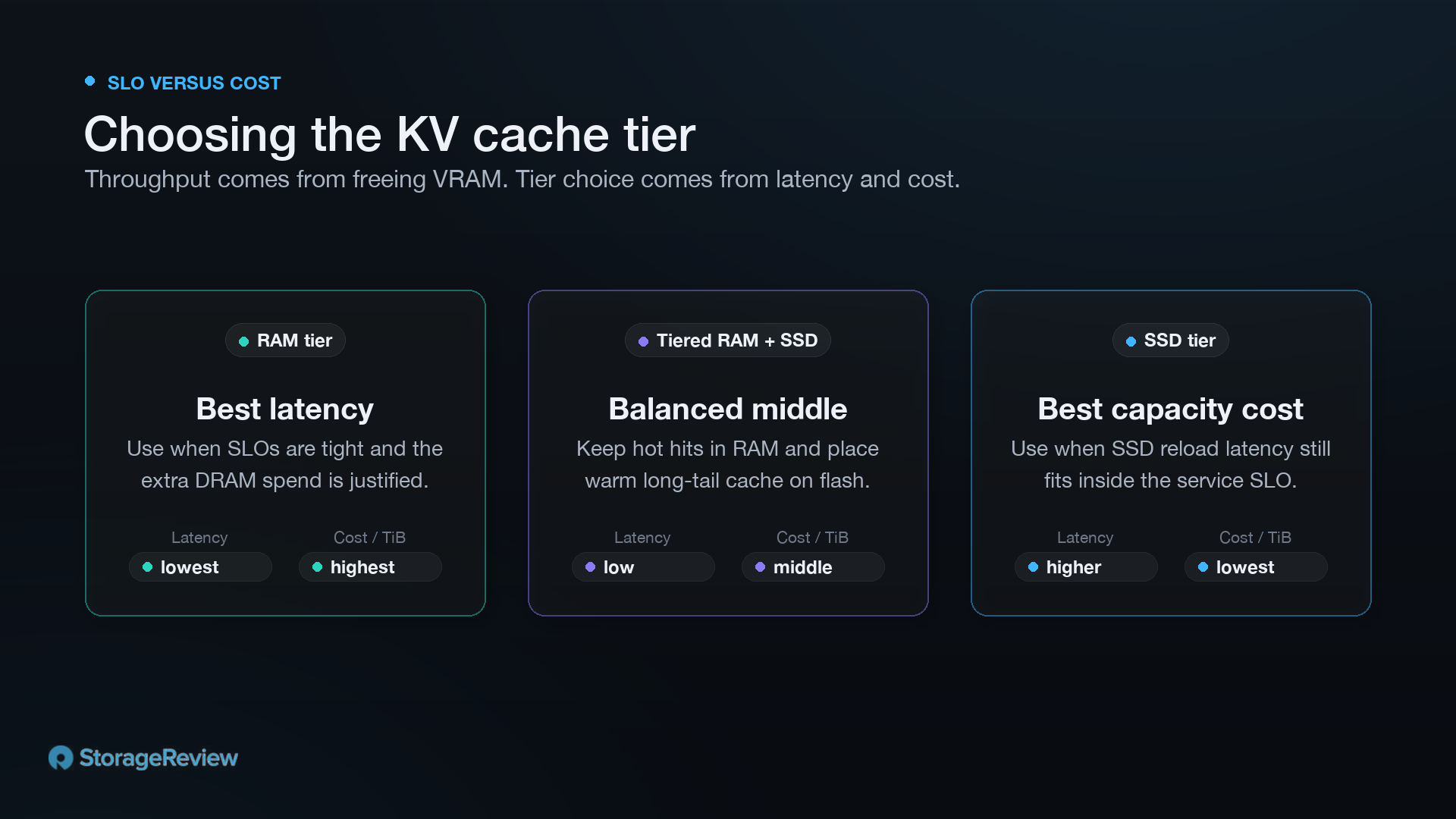
The choice between the two is an SLO-versus-cost trade-off that depends on what the operator is optimizing for. Keeping the entire offloaded cache in RAM yields the best latency, but it is a lot of CAPEX for a relatively small latency uplift over flash. Tiering is the middle ground: a smaller RAM tier that absorbs latency-critical hits where they matter, with a storage tier behind it that holds the warmer long-tail caches that do not need to come back within a few hundred milliseconds.
Another way to think about KV caches is by their size. Sizing the storage tier comes down to the maximum token throughput the setup can sustain. The KV footprint a system has to retain is the throughput times the TTL of cache entries. Every produced token writes a KV entry, so the math is just the rate at which tokens arrive times how long they are kept. The two TTL defaults in production are five minutes and one hour.
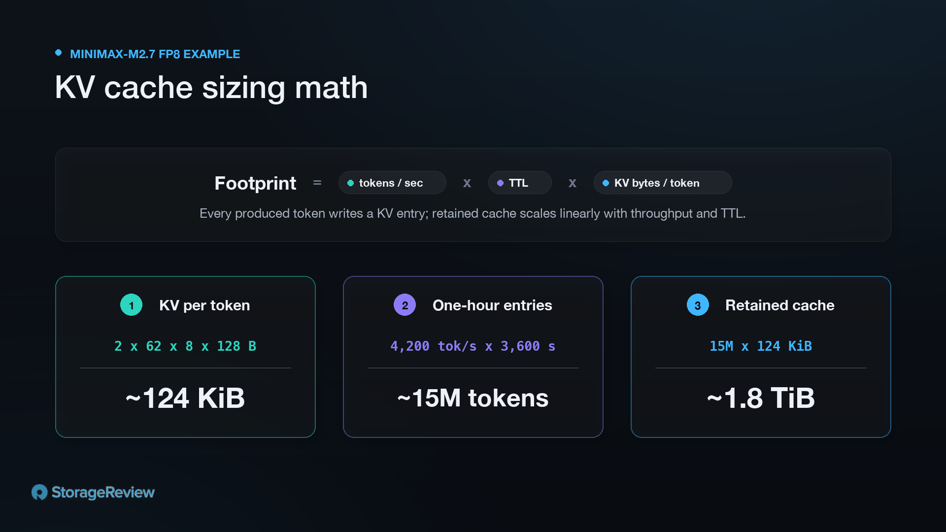
Let’s work out the KV cache size for MiniMax-M2.7 in FP8, as tested here. At one byte per KV element, the per-token entry is 2 × 62 × 8 × 128 bytes, or roughly 124 KiB. This generalizes to any grouped-query-attention transformer: per-token KV is layers × KV-heads × head-dim × 2 (for K and V) × dtype-bytes, so a model with more layers or KV heads writes proportionally more per token. At the moderate operating point here (roughly 4,200 tokens per second on the RAM tier), an hour of retention produces about 15 million tokens of cache, which at 124 KiB per token is about 1.8 TB. That is a lot of DRAM, and it drives up the build cost.
With that in mind, the SLO requirements and the budget guide the choice of tier. If the SLO is loose enough that the SSD-tier reload latency lands inside it, the second tier of KV cache can sit on storage alone, with only the thin RAM staging buffer the connectors require in front of it. The storage cost is modest: peak KV traffic during all our testing was 4.1 GB/s write at the moderate operating point and 1.1 GB/s read, against an fio-measured ceiling of roughly 114 GB/s. The RAID10 array we used had bandwidth to spare by a factor of about 28, so flash stays well clear of being the bottleneck even as the XE7740 scales toward its full eight GPUs and takes on more concurrent load. That headroom is what lets an operator provision the tier for capacity rather than speed. Every added terabyte of D7-PS1030 extends the TTL and the working set the system keeps resident, and a larger resident cache means more avoided recompute and more tokens served.
Endurance is the constraint that defines this tier. A KV offload cache is very write-intensive: every token the model produces writes a KV entry, and TTL churn keeps rewriting the tier around the clock, so the drives effectively never stop taking writes. Across our eight-drive array, sustained writes ran 1.9GB/s, and under the RAID10 layout we tested, mirroring doubles what the media absorbs, which works out to roughly 3.2 drive writes per day on each 12.8TB drive, slightly above the D7-PS1030’s 3 DWPD sustained rating. For primary storage that would be disqualifying, however that is acceptable in this case. The cache is disposable by design, and the failure mode of a worn drive is recompute, not data loss. RAID0 is arguably the better fit for this tier for some, striping across all eight drives so nothing is written twice and cutting the media rate to about 1.6 DWPD, comfortably inside the rating. Either way the conclusion holds: this workload consumes endurance faster than anything else in the box, dedicated high-endurance drives carry a fraction of the capacity the tier needs, and that combination is what makes a write-focused, high-capacity drive like the PS1030 the right choice.
Tokens Per Dollar
The performance section showed that flash retains most of the throughput and maintains first-token latency that DRAM cannot once the working set outgrows memory. What makes that matter commercially is the cost of the tier doing the holding. The easy fix for recompute is to buy more of that expensive DRAM in the system; the offload argument only works if the storage tier is meaningfully cheaper per unit of capacity.
The clearest version of the gap is capacity, not price. The 512GB DRAM offload tier is the one that filled and began evicting; the flash tier, measured in terabytes, is the one that did not. No practical DRAM budget can put tens of terabytes of KV cache next to the GPUs, so past a certain context length, the decision is not fast DRAM versus flash; it’s flash versus discarding the context, which is the eviction that costs throughput and latency in the first place.
On price, enterprise flash has long sold at a fraction of DRAM’s cost per terabyte, a structural gap that follows from NAND’s multilevel, 3D-stacked cells versus DRAM’s one-transistor-one-capacitor design. The 2026 memory crunch has pushed both up sharply, and NAND contract prices have been climbing at least as fast as DRAM through the year, so this is not a case of flash getting cheaper while DRAM spikes. Even at today’s inflated levels, though, the per-terabyte gap persists, and flash remains the only tier where terabyte-scale cache capacity is available at a cost that fits a serving budget.
Throughput and cost point the same way. At the crossover where flash pulled ahead, it was sustaining more tokens per second than the DRAM tier, not fewer, so it is not trading throughput for capacity but delivering more of it on media that costs less per terabyte. On a tokens-per-second-per-dollar basis, that is a wide margin in flash’s favor, and it widens the longer context has to be retained, since that is exactly where DRAM runs out and flash does not.
DRAM remains the right tier while the working set fits it, and the thin RAM staging buffer the connectors require still sits in front of the flash. But adding more GPUs or more DRAM costs the most per terabyte to buy the peak performance the workload only needs, until the cache fills. Offloading or tiering to flash keeps most of that performance while holding context indefinitely, at a per-terabyte cost that makes it affordable. The final decision, however, ultimately comes down to SLO requirements for the workload the operator is optimizing.
Conclusion
For inference workloads, tokenomics is the entire conversation. The token is the product, and recompute is waste: the GPU has already produced that context once and is being made to rebuild it. Agentic serving is where the stakes run highest, since our week of instrumented Claude Code traffic showed 98.16% of tokens were cache reads, context the GPU had already computed and would otherwise rebuild on every eviction. KV cache offload turns the prefill compute that would have gone to rebuilding that history into new tokens instead. On the XE7740, that showed up as up to 2.9X the total serving throughput of the VRAM-only baseline under heavy load, with the model, GPUs, and engine held constant. Where the DRAM tier filled and fell back, flash held that throughput with capacity DRAM can’t match.
None of this ends the need for DRAM, though. For short, bursty workloads, where a session opens, runs briefly, and closes before its cache outgrows memory, DRAM is the right tier, and KV cache offload adds little. The working set fits, the latency is the best available, and there is nothing to evict.
But we see that profile as the exception, where only a DRAM tier is sufficient. Most production inference now runs long and runs continuously: multi-turn agents, large contexts, steady concurrency, users who return to the same session. There, the working set outgrows any memory tier an operator can afford to provision, the cache is evicted, and the GPU is put back to work rebuilding context it already produced. That is the expensive failure mode, and it is common.
For those workloads, offloading the KV cache to flash pays off on two fronts. It keeps the GPUs producing new tokens instead of recomputing old ones, which is the tokenomics efficiency this whole exercise measures, and it puts the capacity that makes that possible on the most cost-effective durable tier in the system. The consequence that matters most on a build sheet is what it removes: a server that leans on flash for cache can be specified with far less DRAM, and with memory priced as it is in 2026, that is one of the largest savings available in the quote. The token is the product, and for the long-context workloads that now dominate serving, the token-efficient path is the one that stops paying to produce the same tokens twice, and that path runs through flash.
Solidigm SSD Storage for AI
This report is sponsored by Solidigm. All views and opinions expressed in this report are based on our unbiased view of the product(s) under consideration.


 Amazon